
In endurance sports physiology, the ideas of critical power and, in running, critical speed take up a lot of space. Without judging whether it makes sense in cycling or other sports, the critical speed concept in running is, in any case, a flawed approach. That is the conclusion of a scientific paper published by Spanish researchers in 2022.
The concept of critical power was developed in 1965 thanks to the work of Monod and Scherrer. It only became popular much later in running, largely driven by the commercialization of Stryd running power meters, which can estimate your critical power.
Running power, measured in watts, represents the effort you produce to move forward. On flat, firm ground, and with no wind, if you keep the same speed, your power output stays essentially constant. In flat running, critical power can therefore be treated as equivalent to critical speed.
That is not necessarily true in cycling, where if the rider stops pedaling (zero power), speed is not zero, especially downhill.
Contents
The definition of critical speed
The critical speed model assumes, incorrectly, that there is a hyperbolic relationship between average speed and time for maximal efforts lasting between 2 and 15 minutes.
A runner’s critical speed is determined from all-out efforts performed on different days, over durations between 2 and 15 minutes. In practice, that could be something like racing a 1500 m and a 5000 m flat out.
From those two results, you can plot average speed as a function of time to exhaustion. Thanks to the “magic” of hyperbolic relationships, you can linearize distance versus time and draw a straight line through the points. The slope of that line is then called critical speed.
The original critical power concept proposed in 1965 by Monod and Scherrer states that critical power is the power you can sustain “for a very long period without fatigue”, or later, as some put it, “almost indefinitely”. Half a century later, physiologists still lean on that definition.
I don’t know about you, but for me a speed you can hold without fatigue is something you can cruise at for 5 to 6 hours, basically easy endurance running. Yet, in most scientific papers, critical speed calculations end up matching an intensity you can sustain for only 20 to 60 minutes at best. That sounds much closer to an anaerobic threshold type of effort, where you have to work, than to an “easy” pace.
Track races and personal bests, either over a season or across an athlete’s career, make it easy to compute critical speed. And you quickly notice it works only so-so, because depending on which distances you use, critical speed changes quite a bit.
An example of calculating critical speed for a runner
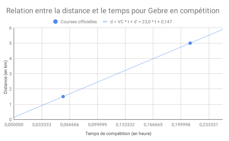
According to the critical speed model, if you draw the line between two points close to 2 and 15 minutes, here the 1500 m and 5000 m, you get the following equation:
d = CS * t + d’
In the case of Ethiopian runner Haile Gebreselassie, critical speed (CS) is 23.0 km/h and d’ = 0.147 km, sometimes called anaerobic distance capacity (ADC). According to the model’s authors, this would be the distance you can run using only your anaerobic reserves.
This distance equation can also be expressed in terms of speed by dividing distance by time. You get:
v(critical speed) = CS + d’ / t = 23.0 + 0.147 / t
Or better, using a race distance: v(critical speed) = CS / (1 – d’/d)
So Haile Gebreselassie should be able to run at 23 km/h for a very long time. If he runs for one hour (t = 1), he should manage 23.147 km/h. But “Gebre’s” one-hour best is 21.29 km/h, as shown below.
“Gebre” runs 5 km at 23.7 km/h and 10 km at 22.75 km/h. So this “critical speed” could only be held for about twenty minutes by the Ethiopian. That is a long way from a speed you can sustain for a very long period without fatigue. Is the critical speed model actually coherent?
The 4 limitations of the critical speed concept listed in the Spanish paper
- The inconsistency of the experimental evidence supporting the classic definition of critical power and critical speed.
- The wide range of relative intensities at which critical power and critical speed have been identified as occurring.
- The arbitrary choice of trial durations used to assess critical power and critical speed.
- The inappropriate choice of a hyperbolic function model to describe the relationship between speed and time.
It is simple, physiologists do not agree on which time trials you should use. Some publications recommend one time between 2 and 3 minutes, and a second between 10 and 15 minutes. Others recommend a second time around 20 minutes, and sometimes even beyond 40 minutes.
If a true hyperbolic model really held from 2 minutes to 1 hour, the slope of the line would not be sensitive to these differences, because the calculated critical speed would be identical regardless of which longer effort you choose.
To test whether the chosen distances influence critical speed, the Spanish researchers used 2019 race results from 10 national-level male and female athletes, each with a result over 1500 m, 3000 m, 5000 m, and 10,000 m.
If you use only the 1500 m, 3000 m, and 5000 m, you get an average critical speed of 19.6 km/h (96.9% of the average speed over 5000 m). But if you add the 10,000 m, average critical speed becomes 18.7 km/h (97.7% of the average speed over 10,000 m). Critical speed depends first and foremost on the longest distance selected for the calculation, as we will also see later with Haile Gebreselassie.
What is more, in the scientific literature some authors state that critical power can be very low, under 40% of maximal power. Others claim critical speed is close to vVO2max, or even above it. That huge spread comes from an inconsistent definition of critical speed.
So how should you model running speed?
The hyperbolic model is a power-law relationship between time and power. The landmark study using this model dates back to 1925, a time when French runner Jean Bouin held the one-hour world record with 19,021 m and when longer distances were rarely raced.
In reality, with my former CNRS/MIT colleagues, we showed in 2018 that modeling performance using a logarithmic representation of time and power produced much better results, especially for the half marathon and marathon.
The example of Haile Gebreselassie’s personal bests, a former world record holder over 5000 m and 10,000 m and an elite marathoner, from 3000 m to the marathon, is striking. For the calculations, all performances from 3000 m to marathon were used, not just the 1500 m and 5000 m above. Keeping the 23.0 km/h critical speed calculated earlier was of limited value because every performance would have been faster than 23 km/h, making the model look even worse.
The table below shows his actual speed (2nd column) for each personal best, then the speed estimated via critical speed (3rd column) and the speed estimated via the CNRS/MIT model (5th column), along with the percentage gap between theory and reality.
Haile Gebreselassie was chosen because he raced a wide range of distances with a career spanning track and road, a bit like marathon world record holder Eliud Kipchoge.
A positive percentage (columns 4 and 6) indicates the runner ran slower than predicted, meaning that relative to his other performances, that distance was less optimized. A negative percentage means the runner beat the predictions and therefore represents one of his best performances.
The critical power model does better than our CNRS/MIT model only over 15 km and 25 km (-0.60% and 0.10%), two distances that are rarely raced. Here, the CNRS/MIT model is actually more coherent because the 1.23% and 0.79% show those two performances were not optimized (positive percentage), on two distances that are not common competitive targets. He even ran faster over 10 miles (16.09 km) than over 15 km, which suggests his 15 km result is relatively average for him (still exceptional for most runners).
The CNRS/MIT model shows that “Gebre’s” best performances are over 5000 m and 10,000 m, which is exactly what you would expect since those were world records at the time.
For the summary table below, speeds were calculated using the official distance as the input parameter.
| Distance (km) | Actual speed (km/h) | Speed (Critical model) | v(CS) / v – 1 | Speed (MIT / CNRS model) | v(MIT) / v – 1 |
| 3 | 24.26 | 28.62 | 17.93% | 24.30 | 0.16% |
| 3.22 | 24.08 | 27.83 | 15.57% | 24.20 | 0.49% |
| 5.00 | 23.70 | 24.54 | 3.55% | 23.54 | -0.70% |
| 10.00 | 22.75 | 22.18 | -2.49% | 22.50 | -1.10% |
| 15.00 | 21.62 | 21.49 | -0.60% | 21.88 | 1.23% |
| 16.09 | 21.74 | 21.40 | -1.60% | 21.78 | 0.15% |
| 20.00 | 21.51 | 21.16 | -1.61% | 21.45 | -0.26% |
| 21.10 | 21.48 | 21.11 | -1.76% | 21.37 | -0.54% |
| 21.29 | 21.29 | 21.10 | -0.87% | 21.35 | 0.33% |
| 25.00 | 20.94 | 20.97 | 0.10% | 21.11 | 0.79% |
| 42.195 | 20.42 | 20.66 | 1.17% | 20.32 | -0.50% |
In this Gebreselassie example, and to extend the Spanish paper, you can also see that the more races you include when computing critical speed, the lower critical speed becomes (the 2nd row uses the first two distances, the 3rd row uses the first three, and so on). Critical speed ends up between 20.23 km/h and 22.96 km/h, which is more than an 11% spread. Which one should you trust?
| Distance (km) | Actual speed (km/h) | Critical speed (km/h) |
| 3 | 24.26 | – |
| 3.22 | 24.08 | 21.82 |
| 5.00 | 23.70 | 22.96 |
| 10.00 | 22.75 | 22.14 |
| 15.00 | 21.62 | 21.13 |
| 16.09 | 21.74 | 21.12 |
| 20.00 | 21.51 | 21.03 |
| 21.10 | 21.48 | 21.00 |
| 21.29 | 21.29 | 20.92 |
| 25.00 | 20.94 | 20.72 |
| 42.20 | 20.42 | 20.23 |
I hope this article helped you see the limitations of critical speed, and made you want to dig deeper into the topic with the two readings below, two scientific papers (in English) that are available for free.
If you use running power, there is no need to throw away your Stryd sensor. Even if the critical power concept is not very coherent, the power-duration curves you can generate should still help you estimate the power you could sustain for a given time. That can be useful for endurance training and pacing strategy.
You can also estimate your next race performances with our online running performance predictor, based on the CNRS/MIT model.
Running power is especially useful on hilly routes and can help you manage your effort and improve pacing. If you use critical power in your training and it works well, it is very likely that the critical power provided by Stryd is close to your anaerobic threshold power, which in theory can be sustained for 40 minutes to 1 hour. If you train using percentages of critical power or percentages of anaerobic threshold power, you will end up with very similar target powers.
The paper that challenges the critical power concept in running:
Gorostiaga EM, Sánchez-Medina L, Garcia-Tabar I. Over 55 years of critical power: Fact or artifact? Scand J Med Sci Sports. 2022 Jan;32(1):116-124.
The paper presenting running performance modeling with a logarithmic representation of time and speed:
Mulligan M, Adam G, Emig T. A minimal power model for human running performance. PLoS One. 2018 Nov 16;13(11):e0206645.